The naïve interpretation of a machine learning model’s predictions is some form of additive effect of its features. However, in the real world, interactions between features must also be taken into account. Consider a model that predicts how patients will react to a new treatment. Different features such as age and weight could affect the outcome. There might be, for example, minimal risk to prescribe the treatment for people over the age of 40 or for overweight patients. However, age and weight might interact and giving the treatment to an overweight patient over the age of 40 might be fatal.
In this article, we will discuss how to detect feature interactions using Friedman’s H-statistic. We then move onto another method that can detect feature interactions based on a specific model’s performance, thus helping to also explain the model.
How to detect feature interaction
One of the basic methods for detecting interactions is the Friedman’s H-statistic. This method uses the notion of the partial dependence function [1], which is the marginal effect of a set of features on a model prediction. The method compares the observed partial dependence function to the partial dependence function under the assumption that there are no interactions. A large difference between the two implies that there are interactions.
H-statistic [2] can be computed in two ways: The first gives a measure of the interaction of a single feature with all other features, while the second gives a measure of the interaction between two features. The H-statistic’s value is between 0 and 1, where 0 means no interaction and 1 means that the effect of the feature (or features) on the prediction is only due to the interaction. A common approach is to select the most highly interactive features using the first method of calculation and then investigate the interactions of all the feature pairs that contain one of these interactive features using the second method.
A disadvantage of H-statistic is its costly calculation time, as it relies on partial dependence function values (for each value the model needs to predict across the whole dataset). In the next section, a different approach for estimating feature interaction will be introduced which is much faster to calculate.
Feature Interaction based on Model Performance (FIMP) [3]
We will now delve into another method that tries to measure the interaction by determining the variance between the model’s conventional prediction performance and its performance when only the individual feature effects are considered. To neutralize the influence of a given feature in a prediction model, we will shuffle its values.
We will note by the prediction performance of a fitted model on a dataset . This can be any performance measure suitable to the prediction task at hand. For classification tasks, measures such as accuracy or Area Under the Curve (AUC) can be used, whereas for regression tasks the RMSE is a popular choice. Next, the notion is used to refer to a copy of the dataset where all the features are randomly shuffled. measures the impact of feature on the model’s performance and is given by:

The logic is that the larger the feature’s influence on the model’s performance, the more that neutralizing it (using shuffling) will lower the model’s performance, and therefore will lead to a larger . In the same way, refers to the impact of both i and j on the model’s performance.
The Feature Interaction based on Model Performance (FIMP) between features is defined as:

FIMP will have a value of 0 when there is no interaction between features i and j A positive interaction implies that the relationship between the features increases the prediction performance, while a negative interaction leads to a decrease in the performance.
A simple example
To demonstrate how to calculate FIMP we will use a synthetic dataset using the following formula given by Friedman:
![]()
All the features are independent and uniformly sampled between 0 and 1. is a standard normal noise term. The label for the dataset will be 0 or 1 depending on if the F value is below the average of F across the dataset or not, respectively. Note that there is only one interaction between and . In addition, the features do not affect the predicted label at all. We train a simple MLP model on this dataset that tries to predict the label.
To calculate FIMP we can simplify its formula to the following:

The original paper describing the FIMP method [3] does not explain how to calculate the interactivity of a single feature against all other features like is done for the H-statistic. We achieve this by considering the second feature as the set of all features except . We therefore can define:
![]()
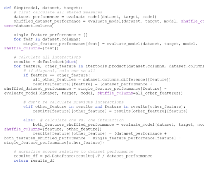
The following code is a simple implementation of FIMP in Python that returns a matrix with all the interactions between feature pairs. The diagonal of this matrix is the interactivity of each feature:

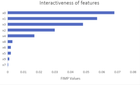
By plotting a bar chart that shows the interactivities of the features in our synthetic dataset we can immediately see that are the most interactive features followed by features .
![]()

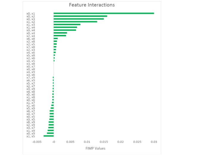
Now that we found the most interactive features, we can drill down more and calculate FIMP for two-feature interactions:

The real interaction between and is clearly visible from the chart compared to all other possible interactions. In addition, all the features that do not affect the label at all (features x5– x9) and therefore their FIMP interactions are close to 0, meaning no interaction.
To summarize, by using FIMP we are detecting the interactions that are implied by the model’s performance. This gives us an explanation of how the model’s prediction (in this case an MLP network) is affected by the different interactions of the features. In addition, the calculation time for all the interaction pairs is considerably short compared to the time it takes to calculate H-statistic.
References
[1] A. Goldstein, et al., Peeking Inside the Black Box: Visualizing Statistical Learning with Plots of Individual Conditional Expectation (2014). https://arxiv.org/pdf/1309.6392.pdf
[2] C. Molnar, Interpretable Machine Learning (2021) https://christophm.github.io/interpretable-ml-book/interaction.html
[3] Oh, S. Feature Interaction in Terms of Prediction Performance. Appl. Sci. 2019, 9, 5191. https://doi.org/10.3390/app9235191