Why should I trust your explanations? A more critical outlook at the most common explainability methods, their advantages but also limitations. As the demand for explainability rises, more and more companies, professionals and organizations introduce some of the methods to produce explanations for their models. However, do these methods deliver? Can we trust their results?

In this blog post as well as in an additional blog post that was already published we aim to survey the existing methods for non-linear model explainability, focusing on the practicalities, limitations and mostly on the out-of-the-box behaviour of the existing implemented methods. In the current blog post we will focus on local explanations.
Link to the previous blog post that dealt with Global explainability can be found here.
As mentioned in the previous part, explainability methods can be roughly divided into global and local explanations. While saying something on the model as a whole makes more sense when we are in research and development stages, and probably mostly useful for professionals, such as Data scientists, local explanation is also meant for the end users. These could be the regulators, companies, or the people benefiting from the model’s predictions. This means that giving the correct explanation is not enough. You also need it to be clear and easy to understand for humans (you can read more about what constitutes a “good” explanation in Miller’s review (1)). And importantly, when explanations are produced for regulatory purposes you need it provide some guarantee that what you see really explains the prediction.
In this blog post I will discuss the two most popular existing local explainability methods:
A notebook with all the code used in this post can be viewed here.
Model and Data
The data I will be using for this part is the classic “Titanic: Machine Learning from Disaster” from Kaggle. More details about the dataset can be found here. The preprocessing stages of the data I employed are very basic and can be viewed in the repository linked above.
The model I chose to use is XGBoost. It is a decision tree based ensemble model. A brief explanation about tree ensemble models and boosting can be found in part I of this series.
The full XGBoost class, which also includes hyper parameter search using Bayesian optimization can be found here. The current usage of the class:
LIME
Much has already been written and said about LIME. I won’t go into many technical explanations, these can be found in many other sources (for example in this great book or in the documentation). But rather briefly, I will explain the basic idea and move to practical applications and limitations.
In general the idea is straightforward: the entire space of the problem is complex and thus can’t be modeled by a simple linear model, so we instead train a higher capacity “ black box” model. However, given a specific instance (sample) and a small environment around it, we can perhaps assume local linearity, train a linear simple model on this local environment and produce an ‘instance related’ explanation. This simple linear model is called a surrogate model.
The data for the local training is obtained by permuting the instance of interest we want to explain. The samples generated are weighted by their distance from the original sample using euclidean distance metric. The labels are obtained by probing our black box model.
One very important thing to remember is that the surrogate model is an approximation of our model and not an exact replica. Since (a) local linearity is an assumption and (b) We produce a separately trained model with K features, N samples and labels from a distribution different than the ground truth. The original model and the surrogate model don’t always produce the same prediction.
Let’s apply the LIME explanations to a couple of examples from our test data.
Theoretically, using LIME can be as easy as running these two lines:
However, to run LIME with XGBoost we need to produce a wrapper class (main function in the repository) that handles some of the input-output matching.
The class usage for the following plots:
> Sample #4: Male, Age = 27, Title=Mr … Didn’t survive
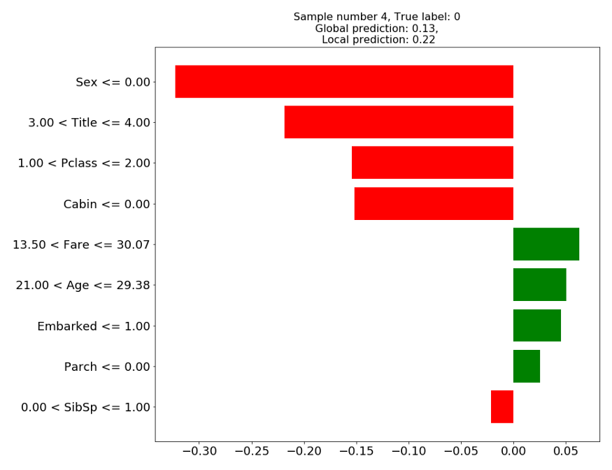
Figure 1: LIME explanation on test sample 4
In figure 1, we can see that the prediction of the local linear model (0.22) is relatively close to the prediction of the global model (0.13). According to the local model, the prediction of the death of this gentleman was mainly due to him being a “he” and a “Mr”, and belonging to class C, while his age would have worked in his behalf. Finally, his family status (Parch, SibSp) seem to play a very little role in the prediction.
The explanations are not very clear-cut, especially for the continuous features. While being 27 years old might seem to be helpful in surviving, does it mean that being older or younger is worse? and by how much?
Let’s look at another example:
> Sample #35: Male, age = 11, title=Mr … Didn’t survive
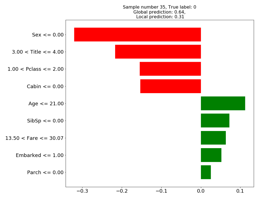
This case demonstrates the possible mismatch between the local prediction (0.31) and the global prediction (0.64). In fact, it might seem that the local model is more accurate than the global model, since this individual according to the true label didn’t survive. The fact that our surrogate model is “correct” while our XGBoost model is “wrong” is a coincidence, not a feature.
The surrogate model should be explaining the prediction of our complex model, regardless of it being right or wrong. Before we even start thinking about the correctness or quality of the explanation, it is essential that their prediction will be the same.
Another potential weakness of the LIME method is the need to manually pick the number of features that out surrogate model will train on, and the size of the kernel that defines our local environment size.
Theoretically, the LIME optimizer should be minimizing complexity, and thus the number of features, while simultaneously minimizing the loss, resulting in some optimum number of features. Practically, we need to pass the number of features (K) to the model. This has an effect on the stability of the explanations, as can be demonstrated below:
Sample #42: Female, age=63, title=Mrs … Survived
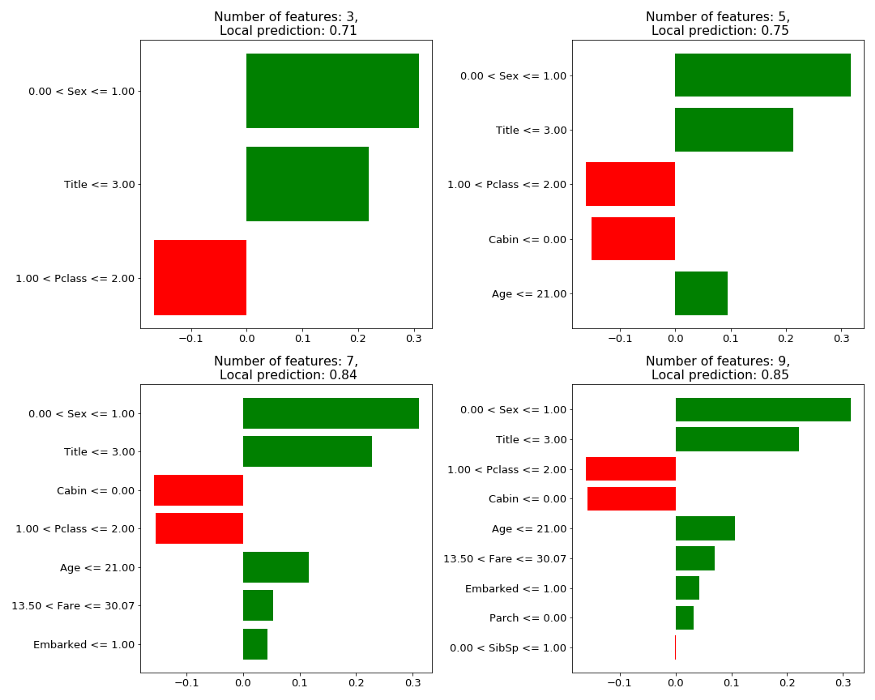
Figure 3: LIME explanation on test sample 42 with different K’s
It appears that changing K has potentially two effects on the results: (1) It can change the local prediction value slightly, and (2) It can change the top selected features, as can be noticed when shifting from 5 to 7 features. The third feature in importance when choosing K=5 is “Pclass” while when choosing K=7 the feature “Cabin” is taking this place and pushing “Pclass” one place down.
Partial explanation for the phenomena are feature dependencies. Some features can be “good” predictors only when combined with other features. Thus only when “enough” features are allowed to the training the combinations are possible.
Since K is manually given this lack of stability is a major weakness. For the same trained model and test set, using a different K can potentially change the explanation (especially if it is built on a subset of the top X features).
While it is straightforward, easy to understand and relatively easy to use, LIME suffers from a number of disadvantages. Namely, the local linearity assumption, the need for manually defining K number of features to use and mainly the potential inconsistency between the surrogate model prediction and our complex model prediction. Finally, the values LIME outputs seem to be lacking comparative value and meaning. What does the value per feature represents? What is the relation between these values and the local model prediction? Given multiple samples, can anything be deduced looking at the values of their features in LIME?
SHAP
SHAP is a local explainability model that is based on the shapley values method. Shapley values method is a game theory method with theoretical basis that suffers mainly from being computationally expensive.
SHAP solves this problem by proposing two sub-methods: KernelSHAP and TreeSHAP. Since we are trying to explain our XGBoost model it makes more sense to use the TreeSHAP model. But first, I will briefly explain the Shapley values method and the main innovations in SHAP.
In Shapely values we treat our features (or their combinations) as players. These players can form “coalitions” and play games. The outcome of a game is our prediction. Our goal is to calculate the average contribution of a feature to the predictions of different coalitions in comparison to the average prediction across all instances. The shapely value is the contribution that comes from this feature. However, going over all coalitions scales exponentially with the increase in the number of features.
This is where SHAP is suppose to help.
KernelSHAP views the solution as a combination of previously introduced LIME and Shapely values. The idea is to train a surrogate model to learn the shapely values of different coalitions as it’s weights. In different permutations some features are absent. The absent feature is replaced by a sample from it’s marginal distribution (much like in the global permutation method described in part I). Unlike LIME the coalitions are weighted not according to a distance metric (euclidean) but according to the coalition theory (large and small collations are more important).
We won’t be dealing with KernelSHAP in this blog post, but it is important to note that it suffers from a major disadvantage typical to permutations methods: it disregards any dependencies between features when permuting an absent feature, thus producing many non realistic combinations. Furthermore, while many companies treat SHAP values as if they were shapely values and thus have mathematical guarantees on their correctness, KernelSHAP is an approximation method, and does not give exact values.
TreeSHAP proposes an algorithm that grows at a polynomial rate with the number of features. In addition, the additivity characteristic of the Shapley values means that we can compute the shapely value of a tree ensemble by weighted average of the individual trees. The TreeSHAP algorithm takes only “allowed” paths within the tree, meaning it doesn’t include non-realistic combinations as in the permutations methods. Instead, it takes the weighted average of all the final nodes that were “reachable” by a certain coalition.
Let’s look at a similar example as in LIME and use TreeSHAP to explain the prediction.
> Sample #35: Male, age = 11, title=Mr … Didn’t survive
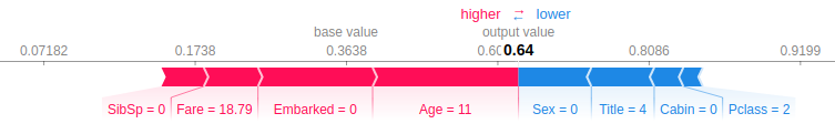
The red arrows represent the features that drive the prediction higher, while the blue arrows represent the features that drive the prediction lower. The base value is the average of all predictions. The output value is the global model output. The value next to each feature is the actual input value of this feature in the sample of interest, and not the shapley value! Finally, while the size of the arrows is proportional to the magnitude of the pushing force, they are actually scaled using log-odds and not probability. More about this below.
Looking at this specific example we can detect two major differences from the LIME prediction:
- SHAP explains the prediction of our model. Meaning, it doesn’t train another model and thus there is no danger in having our explainer predicting and explaining a different result.
- TreeSHAP looks at feature importance compared with the general base value, while LIME trains a local model. This means that some features, like Age, might have a considerably different influence when looking outside of the local environment.
SHAP working space: log-odds vs. probabilities
In classification, it is easy to look at the global output as a probability for a class, a value between 0 to 1. However, it is not additive. Thus, TreeSHAP works in the log-odds space, outputting the shapley values as log-odds contributions. Since the output in the log-odds space is hard to interpret, it makes sense to transform it back to probabilities. This is done by using the “link” parameter in the visualization function above and in fact the visualization ticks labels of the force plot are showing probabilities. But this only transforms the axis (which is now not linear and thus unevenly spread), and not the individual SHAP values. If for some reason you need the individual SHAP values of the features, you can only obtain them (at least efficiently) using approximation. You will need to transform the output value and the base value to probabilities and stretch the SHAP values between them.
Note: in the latest release (0.34) an option for model_output=’probability’ was added. Using this option we can transform the SHAP values to probabilities directly using the DeepSHAP re-scaler. However it only works with “interventional” feature perturbation, meaning it uses causal inference rules to break dependencies between features and requires a background dataset.
SHAP global explainability
This section perhaps belongs in the “Part I: global explainability” blog post, but I think it will be better understood here, after reading the explanation on SHAP.
SHAP can be used to make global explanations using the combination or average across all local instances. For this purpose, we can plot a Summary plot using the “bar” option and the “dot” option to produce two types of plots:
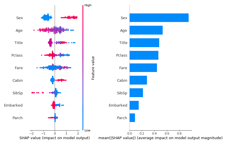
Each dot in the plot on the left is a shapley value in a single instance of a single feature. The color represents the feature’s value in that specific instance. In the right plot we see the average shapley value per feature across all instances. While the plot on the right produces some version of “feature importance” as described in the global explainability part, in this case the importance value represents the extent to which the feature influences the outcome and not the model performance or model construction. The plot on the right however doesn’t show the direction of the influence and moreover, the interaction between the feature value and the feature influence. These can be seen in the left plot. Looking on the left plot we can clearly see that some features (Sex, Cabin etc..) have a very strong association between their value and the influence direction. Another option (somewhat similar to SibSp feature) is to have a strong association between the value and influence magnitude.
Summary
- While relatively straightforward and easy to use, the LIME method can’t be used to satisfy regulators, and should be used with care for end-users aimed explainability. The fact that the surrogate model can potentially explain a different prediction all together is alarming.
- The SHAP method has a lot going for it. First and foremost, it stems from game theory and has a mathematical proof behind it. This is of course very attractive for regulators. Secondly, it explains the prediction itself (not obvious given LIME). Thirdly, at least for TreeSHAP (but not for KernelSHAP), it eliminates the dependencies issue that is a problem in all permutation methods by using only valid tree paths. Finally, the interpretation of SHAP values is relatively intuitive: “how much each feature contributed to drift away from the base value”. With that in mind, not everything is perfect. SHAP explanations are still missing reference to counterfactual explanations (how would changing the feature’s value effect the outcome). In addition, unlike the simple explanation LIME gives, the explanation that SHAP provides includes all features, which is hard for people to understand and use.
- While not reviewed in this blog, LIME and KernelSHAP can also be used for non-structured data such as images and texts. For such data, both models rely on additional strong assumptions and heuristics to produce the features that will be used. Then, permuting this set of features in SHAP is done naively and doesn’t necessarily makes any sense.
- Finally, most methods reviewed in both blog posts treat features as separate independent beings. They fail to address neither feature correlations nor feature dependencies. But while methods like TreeSHAP solve the feature dependencies bias, none of the methods combines more than one feature in it’s explanation. Namely, they ignore the “the whole is greater than the sum of its parts” phenomena. This is a major drawback to all of the explanation methods.
References
- Miller, Tim. “Explanation in artificial intelligence: Insights from the social sciences.” Artificial Intelligence 267 (2019): 1–38.
- https://christophm.github.io/interpretable-ml-book